Ecology Lab 5: Plant Dispersion Patterns-Data Analysis

In this week’s lab me and my lab group studied the characteristics of populations and how the individuals in the populations are arranged in space. We specifically study the dispersion of Dallisgrass. Dispersion of a population is referred to by the arrangement of the individuals in the population and their spacing from one another. There are three properties that determine the spatial structure of a population. Those three properties are dispersion, distribution, and density. This lab focused on the property of dispersion within an area. Some factors than can influence were individuals settle are wind, moisture, sunlight, competition, and predation. There are three types of dispersion patterns. The three types are clumped, random, and uniform dispersion. The clumped dispersion pattern is influenced by social interactions like mating, safety, and resources. The clumped dispersion pattern results in individuals in a population to live close to each other. The uniform dispersion pattern is influenced by intraspecific interactions like territoriality for prey or root space. The uniform dispersion pattern results in everyone in a population to be evenly spaced apart from one another. The random dispersion pattern results in the spatial position of everyone to occur independently of the other individuals. The random dispersion pattern results in individuals within a population to be in certain locations in a random pattern. I think that the dispersion of Dallisgrass will resemble a uniform dispersion pattern. The reason I be live this is because I believe that the Dallisgrass will be relatively equidistant from each other due to competition for root space.

The method that we used to obtain our data for the dispersion of the Dallisgrass was by using the quadrat method. In this method we would use a meter squared quadrat to determine the frequency of individuals in the area that we were studying. In this lab we would take ten different quadrant samples that would all be randomly chosen. The way that the quadrant locations were randomly chosen was by using a random number generator. We would use the random number generator to obtain the number of steps that we would take in a straight line. Then we would get another random number from the number generator and then take that many steps to the right. Then we would place our meter squared quadrat on the ground where we stopped. We would the count the number of Dallisgrass that was located within the meter squared quadrat. This process would be repeated ten times. The study was conducted in the Confederate Cemetery by the University of Tennessee Chattanooga. The cemetery location is relatively flat with many trees that are scattered across the location. There is some areas of shade and some areas of direct sunlight in this location. This location is subject to light human traffic. The statistical methods that were used to analyze the data was the Poisson distribution formula and the Chi-square test. The Poisson distribution formula was used to illustrate how many plants per quadrat would be expected if the distribution was random. The Chi-square test was used to identify if the distribution differs from a random distribution and how much it differs from a random distribution. In the Chi-square test the alpha level of 0.05 was used.

The total number of quadrats sampled in the group data set was 9. One quadrat was not used because it had an outlier that would skew the data. The average number of individuals per plot in the group data set was 4.33. The total number of individuals observed in the group data set was 39. The maximum number of individuals found in a plot was 8. The total number of quadrats sampled in the class data set was 39. One quadrat was not used because it had an outlier that would skew the data. The average number of individuals per plot in the group data set was 4.9. The total number of individuals observed in the group data set was 191. The maximum number of individuals found in a plot was 16.

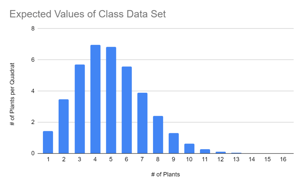
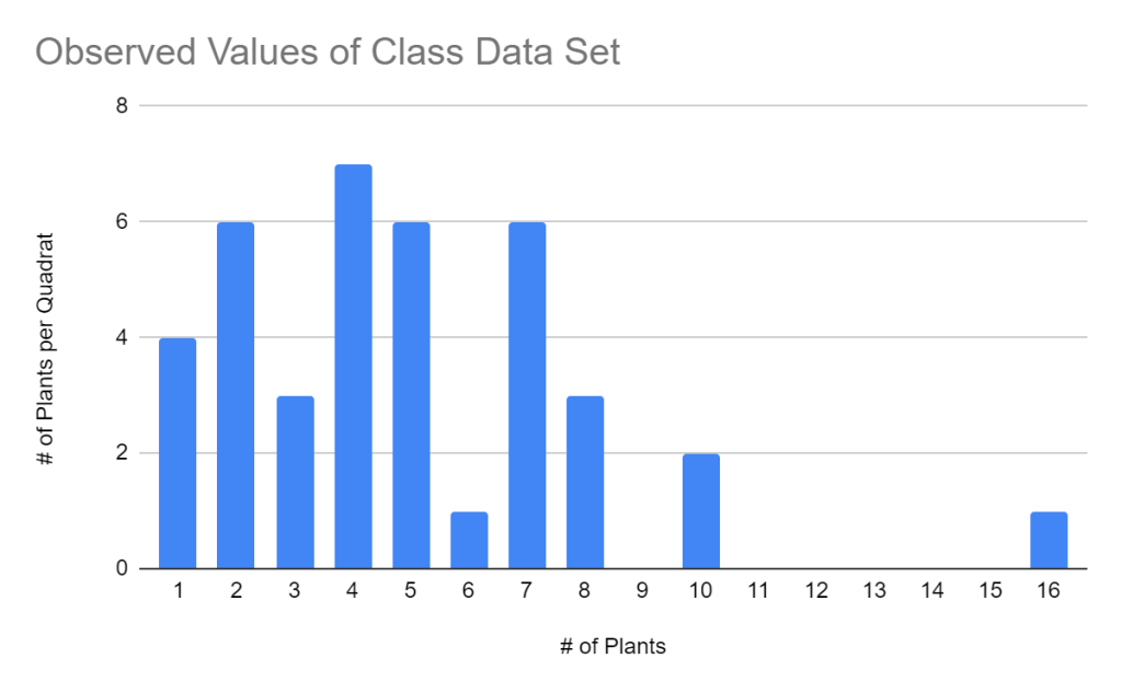
Table 1. This table shows the Chi-square table for the class data set. This table has a sample size of 38 with a critical value of 53.384. The tables calculated critical value is 668.174. This table uses the alpha level of 0.05.

# of Plants/Quadrat	Observed # Plants in Quadrats (O)	Expected # Plants in Quadrats (E)	(O – E)	(O – E)^2	(O – E)^2/E
0	0	0.2904167398	-0.2904167398	0.08434188274	0.2904167398
1	4	1.423042025	2.576957975	6.640712406	4.666560994
2	6	3.486452961	2.513547039	6.317918718	1.812133647
3	3	5.694539836	-2.694539836	7.260544928	1.275001166
4	7	6.975811299	0.02418870075	0.000585093244	0.00008387458015
5	6	6.836295073	-0.8362950733	0.6993894496	0.1023053338
6	1	5.58297431	-4.58297431	21.00365352	3.762090305
7	6	3.908082017	2.091917983	4.376120848	1.119761773
8	3	2.393700235	0.6062997647	0.3675994046	0.1535695235
9	0	1.303236795	-1.303236795	1.698426143	1.303236795
10	2	0.6385860295	1.361413971	1.853447999	2.90242491
11	0	0.2844610495	-0.2844610495	0.08091808867	0.2844610495
12	0	0.1161549285	-0.1161549285	0.01349196742	0.1161549285
13	0	0.04378147306	-0.04378147306	0.001916817384	0.04378147306
14	0	0.01532351557	-0.01532351557	0.0002348101295	0.01532351557
15	0	0.005005681754	-0.005005681754	0.00002505684982	0.005005681754
16	1	0.001532990037	0.99846701	0.99693637	650.3214932
Sum =	668.1738049

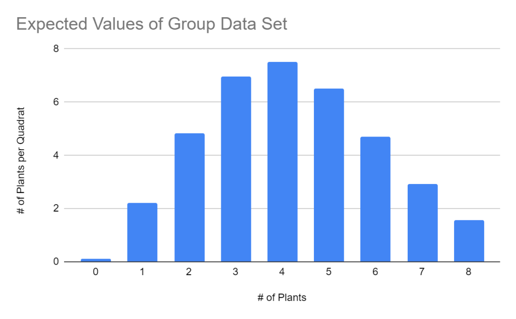
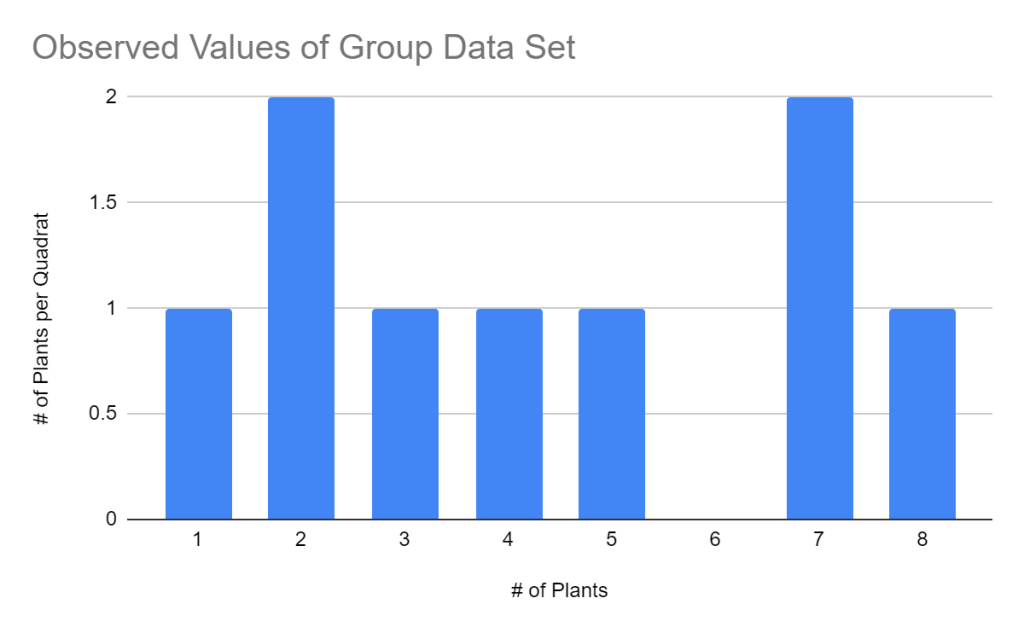
Table 2. This table shows the Chi-square table for the group data set. This table has a sample size of 8 with a critical value of 15.507. The tables calculated critical value is 23.044. This table uses the alpha level of 0.05.

# of Plants/Quadrat	Observed # Plants in Quadrats (O)	Expected # Plants in Quadrats (E)	(O – E)	(O – E)^2	(O – E)^2/E
0	0	0.1185079274	-0.1185079274	0.01404412886	0.1185079274
1	1	2.223603745	-1.223603745	1.497206124	0.6733241602
2	2	4.814102107	-2.814102107	7.91917067	1.64499433
3	1	6.948354041	-5.948354041	35.3829158	5.092273018
4	1	7.52159325	-6.52159325	42.53117852	5.654543805
5	1	6.513699754	-5.513699754	30.40088498	4.667222336
6	0	4.700719989	-4.700719989	22.09676842	4.700719989
7	2	2.907731079	-0.9077310791	0.823975712	0.2833741118
8	1	1.573809447	-0.5738094466	0.329257281	0.2092103855
Sum =	23.04417006

Based on the data that has been collected from the Confederate Cemetery one can conclude that the Dallisgrass illustrates a clumped distribution pattern in both data sets. This means that the null hypothesis that the distribution is random would be rejected. The distribution is identified as being clumped is because the histograms have values far from the mean. This results in the mean being less than the variance. Based on the data my hypothesis is not supported because the histograms do not represent a uniform dispersal pattern. A uniform dispersal pattern would have values close to the mean with short tails. Some factors that would lead to the clumped distribution in the class and group data sets would be that the Dallisgrass grows close together because of mate location of for protection. Another factor for the clumped distribution might be related to high resource concentration in specific areas. The results that were obtained are statistically significant because they illustrate alpha levels greater than the critical value of 0.05. Some environmental factors that could have impacted this study and the data that was collected could be wind, moisture, sunlight, competition, and predation. Comparing the group data set and the class data set it is easier to conclude that the class data set points toward a clumped distribution. The reason it is easier to conclude the distribution from the class data set is because there is more data used in the class data set than in the group data set. Larger amounts of data give a more precise representation of distribution patterns.